Understanding Generative Modeling through transport theory

Generative modeling is often understood as training a neural network with a well-chosen objective function. The key idea is to approximate an unknown distribution $p_{\text{data}}$ with a learnable distribution $p_\theta$. However, the objective function does not really show that we are optimizing a distribution; instead, it mostly looks like we are just optimizing a neural network.

In this article, we will explore the main generative models by analyzing their losses and showing how they optimize a distribution.

Summary

I. Deterministic Transport: GAN and Flows

II. Stochastic Transport

III. Let’s add optimality

Get Started

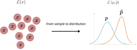
At the beginning, the only thing we have is a finite sample from $p_{\text{data}}$, i.e. a dataset $\mathcal{D}=\{x_i\}_{i=1}^N$, which defines the empirical (discrete) distribution

$$ \hat p_{\text{data}} \;=\; \frac{1}{N}\sum_{i=1}^N \delta_{x_i}. $$

Several ideas have been proposed to approximate $p_{\text{data}}$. A major one is the variational autoencoder (VAE) introduced by Kingma & Welling (2013), which learns a latent-variable model. One assumes a prior $p(z)$ and a decoder (generative) distribution $p_\theta(x\mid z)$, so that the model distribution is

$$ p_\theta(x) \;=\; \int p_\theta(x\mid z)\,p(z)\,dz. $$

Since the true posterior $p_\theta(z\mid x)$ is generally intractable, VAEs use variational inference with an encoder $q_\phi(z\mid x)$ to approximate it, typically a mean-field (e.g. diagonal-covariance Gaussian) family.

However, despite their elegant probabilistic framework, “vanilla” VAEs (mean-field Gaussian posterior, simple Gaussian decoder, etc.) are no longer the dominant approach for high-fidelity generation. At the beginning, the only thing we have is a finite sample from $p_{\text{data}}$, i.e. a dataset $\mathcal{D}=\{x_i\}_{i=1}^N$, which defines the empirical (discrete) distribution

$$ \hat p_{\text{data}} \;=\; \frac{1}{N}\sum_{i=1}^N \delta_{x_i}. $$

A second major idea—central to many modern generative models—is to start from a simple reference distribution $\tilde p$ (typically a standard Gaussian) and learn a transport $T_\theta$ that pushes it forward to the data distribution:

$$ (T_\theta)_\# \tilde p \approx p_{\text{data}}. $$

In other words, generation can be seen as moving probability mass from an easy distribution to $p_{\text{data}}$.

Transport with deterministic path

Transport with deterministic path is the natural formulation of our problem. The key idea is to find an objective to build an application (or a composition of applications) $T$ which transports the noise distribution $\tilde p$ to $p_\text{data}$.

The keyword “deterministic” comes in opposition with “stochastic transport”, where $T$ is no longer an application but a markov kernel.

We have selected two popular examples of deterministic transport: GAN (Generative Adversarial Network) and Normalizing Flows.

GAN

The neural network vision of a GAN is two networks train in competition. A generator $G_\theta(z)$ produces synthetic images from noise and a discriminator $D_\phi(\cdot)$. We feed the discriminator with synthetic images from $G$ and with real images from $\hat p_\text{data}$. The network $D$ try to infer wheter or not its inputs are synthetic or real.

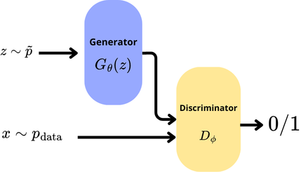
The loss is a min-max objective :

$$ \min_{\theta}\ \max_{\phi}\ \mathcal{L}_{\mathrm{GAN}}(\theta,\phi)= \mathbb{E}_{x\sim p_{\text{data}}}\!\big[\log D_{\phi}(x)\big]+ \mathbb{E}_{z\sim \tilde p}\!\big[\log\!\big(1-D_{\phi}(G_{\theta}(z))\big)\big]. $$

However this formulation is a classic deep learning vision, we build our intuition on the analysis of the objective function. This vision helps to see what task do we use to train each networks, but this suffers of a lack of information on how data are transported from a noise $\tilde p$ to an approximation of the real data distribution $p_\text{data}$.

We aime to reformulate the objective function to extract the learnt transport application.

We readily see that $G_\theta$ is the application which transport noise to $p_\text{data}$. Then we have $x \sim {G_\theta}_\#\,\tilde p$. The optimization to find the correct push-forward becomes :

$$ \mathcal L(D_\phi, G_\theta) = \min_{\theta}\ \max_{\phi}\ \mathcal{L}_{\mathrm{GAN}}(\theta,\phi)= \mathbb{E}_{x\sim p_{\text{data}}}\!\big[\log D_{\phi}(x)\big]+ \mathbb{E}_{x \sim {G_\theta}_\#\,\tilde p }\!\big[\log\!\big(1-D_{\phi}(G_{\theta}(z))\big)\big]. $$

Once set, we want to find a $D^*$ which optimizes $G_\theta$. By using the KKT condition and admitting that each measure are absolutly continuous we show that:

$$ D^*(x) = \frac {p_\text{data}(x)} {p_\text{data}(x) + {G_\theta}_\#\,\tilde p(x)} $$

We reinject this optimum and find that:

$$\mathcal L(D^*, G_\theta) = -\log 4 + \textrm{KL}(p_\text{data}\mid\mid m) + \textrm{KL}({G_\theta}_\#\,\tilde p \mid\mid m), \qquad \text{ where }2m = p_\text{data}+ {G_\theta}_\#\,\tilde p$$

Then the objective on our transport is an optimization in the transport application space with Jensen distance as metric.

This appears to be the Jensen-Shannon divergence, $\textrm{JS}$. This formulation helps to see that GAN are not only an association of neural networks but a real optimization on a push-forward noise to data, in the case of a discriminator perfectly optimized.

This formulation tries to give a theoric objective. In pratice $D$ is not perfectly optimized and $G$ doesn’t follow stricly a minimal $\textrm{JS}$ curve but a neural divergence induced by the network. With a finite capacity for $D$, the class of function possible for $D$, denote $\mathcal F$, is restraint. The neural divergence is not defined from $D^*$ but from a $\sup$ on $\mathcal F$.

$$ \mathcal d(p_\text{data} \mid \mid {G_\theta}_\#\,\tilde p) =\sup_{D\in\mathcal F}\; \mathbb E_{x\sim p_{\text{data}}}\!\big[\log D(x)\big] \;+\; \mathbb E_{x\sim {G_\theta}_\#\,\tilde p}\!\big[\log\big(1-D(x)\big)\big], \qquad $$

Normalizing flows

An other way to transport a distribution is by learning normalizing flows.
The idea this time is to learn explicitly the transport application with an invertible constraint on the transport application.

In GAN we try to descent through a distance (like Jensen-Shannon divergence) to approach a satisfying transport.

However this application often has no density with respect to the Lebesgue measure. Even if such a density exists, GAN do not impose invertibility and do not provide an exploitable Jacobian. As a consequence, the density induced by the generator is intractable.

Normalizing flows take a different point of view. Instead of learning a transport only through a discrepancy between the transported noise and the data distribution, they build a transport map $T_\theta$ such that

$$ (T_\theta)_\# \tilde p \approx p_\text{data}, $$

with the additional assumption that $T_\theta$ is invertible.

As in GAN, we start from a simple noise distribution $\tilde p$, for example a standard Gaussian, and transport it to the data space. The difference is that here the transport application is constrained enough so that we can explicitly compute the density of the transported law. This is the main strength of flows: they do not only generate samples, they also describe how probability mass is deformed by the transport.

If $z \sim \tilde p$ and $x=T_\theta(z)$, then by construction

$$ x \sim (T_\theta)_\# \tilde p $$

Since $T_\theta$ is invertible, one can also go backward from $x$ to $z=T_\theta^{-1}(x)$. This gives access to the density of the transported distribution through the classical change-of-variable formula:

$$ p_\theta(x)= \tilde p(T_\theta^{-1}(x)) \left|\det J_{T_\theta^{-1}}(x)\right|. $$

This formula is central to the flow point of view. It shows that the learnt map is really a transport application: it moves the reference density $\tilde p$ to a new density $p_\theta$, and the Jacobian determinant tells us how volumes are locally dilated or contracted by the map. In other words, contrary to GAN, the transport is not only implicit through samples, but explicit through densities.

In practice, one does not choose any invertible map, because computing the determinant of a generic Jacobian would be too expensive. The idea is then to build $T_\theta$ as a composition of simple invertible applications:

$$ T_\theta = f_K \circ \dots \circ f_1, $$

where each $f_k$ is chosen such that both its inverse and its Jacobian determinant remain tractable.

If we define the intermediate variables

$$ h_0=z,\qquad h_k=f_k(h_{k-1}),\qquad h_K=x, $$

then the density writes

$$ \log p_\theta(x) =\log \tilde p(z)- \sum_{k=1}^K \log \left|\det J_{f_k}(h_{k-1})\right|. $$

This decomposition explains the name normalizing flow: the distribution progressively flows through several simple transformations, and at each step we keep track of how the density changes.

We now want to understand what objective is optimized in this case. Since the model density $p_\theta$ is explicit, the natural objective is maximum likelihood. Given a dataset $\mathcal D=\{x_i\}_{i=1}^N$, we search for the transport application $T_\theta$ which maximizes

$$ \frac1N \sum_{i=1}^N \log p_\theta(x_i). $$

Equivalently, this amounts to minimizing the Kullback-Leibler divergence between the empirical distribution and the transported model:

$$ \min_{T_\theta} \mathrm{KL}\big(\hat p_\text{data}\mid\mid (T_\theta)_\# \tilde p\big). $$

This formulation makes clear that normalizing flows are also transport models. But contrary to GAN, where the transport is learnt indirectly through a neural divergence, here the transport map itself is explicitly constrained and its action on densities is known. The model is not only a generator from noise to data, it is a change of variables between two probability distributions.

Stochastic transport

Instead of learning a single map $T_\theta$ that directly pushes $\tilde p$ to $p_{\text{data}}$, the stochastic viewpoint decomposes the transport into a sequence (or a continuum) of simpler stochastic transformations. This is done by introducing a family of intermediate distributions $(q_t)$ indexed either by a discrete time $k\in\mathbb{N}$ or a continuous time $t\in[0,1]$, with

$$ q_0 = \tilde p, \qquad q_1 \approx p_{\text{data}}. $$

In discrete time, we consider maps $(T_k)_{k=0}^{K-1}$ and define the evolution by repeated push-forward:

$$ q_{k+1} = (T_k)_\# q_k, \qquad \text{so that} \qquad q_K = (T_{K-1}\circ \cdots \circ T_0)_\# \tilde p. $$

In continuous time, we instead describe a time-indexed transformation (a flow) $(\Phi_{0\to t})_{t\in[0,1]}$ and set

$$ q_t = (\Phi_{0\to t})_\# \tilde p, \qquad q_1 = (\Phi_{0\to 1})_\# \tilde p \approx p_{\text{data}}. $$

Define a stochastic dynamic

We call here a stochatic dynamic an SDE that describes how a random variable $X_t \sim q_t$ evolves over time.

Let $X_t \sim q_t$. A general SDE has the form

$$ dX_t \;=\; a(X_t,t)\,dt \;+\; b(X_t,t)\,dW_t, \qquad \text{where } W_t \text{ is a Brownian} $$

In this formulation, defining a transport toward $p_{\text{data}}$ amounts to specifying a family of intermediate distributions $\{q_t\}$, which is implicitly determined by the coefficients $a(X_t,t)$ and $b(X_t,t)$.

Unlike a deterministic transport map, an SDE defines a stochastic transport. In particular, for a fixed $x$ sampled from $\tilde p$, the output of the transport $\phi_{0\rightarrow1}(x)$ may differ across two runs. In this case, $\phi_{0\rightarrow1}$ should be understood as a Markov kernel.

A common strategy is to first define a forward (noising) dynamics that transports $p_{\text{data}}$ to a simple reference distribution $\tilde p$, and then to learn or approximate the corresponding reverse transport starting from $\tilde p$.

The reverse dynamics $d\overleftarrow X_t$ is then derived (or approximated) from the forward dynamics.

This forward–reverse strategy is convenient because it is typically easy to design a forward noising process that maps $\hat p_{\text{data}}$ to a known reference distribution $\tilde p$ (often a Gaussian).

Choose coefficients of the SDE

We choose a linear drift $a(\overrightarrow X_t,t) = -\lambda(t)\,\overrightarrow X_t$ and an isotropic diffusion $b(\overrightarrow X_t,t) = g(t)\,I$.

Why do we start with these forms? As said previously, $\tilde p$ is often chosen to be Gaussian. With a linear drift and an isotropic diffusion, the conditional marginals $\{q_t(\cdot\mid X_0)\}_t$ remain Gaussian and admit closed-form expressions, fully determined by $\lambda$ and $g$.

$$ \overrightarrow X_t \mid \overrightarrow X_0=x_0 \sim \mathcal N\!\big(\alpha(t)\,x_0,\ \sigma^2(t)\,I\big), $$$$ \alpha(t)=\exp\!\Big(-\int_0^t \lambda(u)\,du\Big), \qquad \sigma^2(t)=\int_0^t \exp\!\Big(-2\int_s^t \lambda(u)\,du\Big)\,g(s)^2\,ds. $$

A second question is: why do we include the minus sign in front of $\lambda(t)$?

By analogy with physics, the minus sign makes the deterministic part of the dynamics stable: the drift acts as a restoring force that pulls $\overrightarrow X_t$ toward $0$. Since $\tilde p$ is typically a zero-mean distribution, we want the forward dynamics to have a deterministic component that contracts toward $0$ while noise is progressively injected.

Once $\lambda$ and $g$ are chosen, the forward SDE defines a family of marginals $(q_t)_{t\in[0,1]}$ and therefore a transport from $p_{\text{data}}$ (in practice, from $\hat p_{\text{data}}$) to a simple reference distribution $\tilde p$ (often $\mathcal N(0,I)$). In discrete implementations, we simulate a time grid and obtain a sequence

$$ X_0 \sim \hat p_{\text{data}},\qquad X_{k+1} =\text{forward dynamic}(X_k),\qquad X_K \approx \tilde p, $$

so that the composition of these elementary transitions yields the overall forward transport.

Some examples of forward dynamics

By using the suposition on the SDE coefficients, we build some popular forward process.

• Pure diffusion (no drift): We set the drift (determinist part) as $\lambda(t)=0$. The $\{q_t\mid X_0\}$ familly is gaussian with a variance increasing with respect to the time.
  Indeed, $Var(q_t \mid X_0) = \int^t_0 g(s)^2ds$. The dynamic converges to a gaussian with high variance $\sigma_\text{max}^2$.

• VP-SDE (variance-preserving): We reparametrize $\lambda(t) = \frac 1 2 \beta(t)$ and $g(t) = \sqrt{\beta(t)}$ and take $\beta(t)$ as a positive function.
  As a consequence the law of $X_t|X_0$ converges to $\mathcal N(0,1)$. The name “variance preserving” comes from the conditional to $X_0$ variance converges to 1 and that under condition on $X_0$, variance is contant to 1.

• Ornstein–Uhlenbeck (OU): The process is a VP-SDE but $\beta(t) = \beta$, a constant positive value.

• DDPM (discrete time) dynamics:

  $$ X_{k+1} = \sqrt{1-\beta_k}\,X_k + \sqrt{\beta_k}\,\varepsilon_k,\qquad \varepsilon_k\sim\mathcal N(0,I). $$

  To obtain this dynamic we use a discrete time grid on VP-SDE.

With those forward dynamics, we build $\{q_t\}$ and with them, we transport $p_\text{data}$ - in practice we transport $\hat p_\text{data}$ - to $\tilde p$ (often $\mathcal{N}(0,1)$).

Reverse dynamic

We call a reverse dynamics a dynamics that transports $\tilde p$ into $p_{\text{data}}$. For a forward SDE

$$ dX_t = a(t,X_t)\,dt + b(t,X_t)\,dW_t, \qquad X_t\sim q_t, $$

the corresponding reverse-time SDE (run from $t=1$ down to $t=0$) can be written as

$$ d\overleftarrow X_t=\Big( a(t,X_t)-\Sigma(t,X_t)\,\nabla_x \log q_(X_t)+\nabla_x\!\cdot \Sigma(t,X_t) \Big)\,dt+b(t,X_t)\,d\bar W_t,\qquad\Sigma(t,x):=b(t,x)b(t,x)^\top,$$

and is simulated from $t=1$ down to $t=0$ starting from $X_1\sim\tilde p$.

Here we assume that $a$, $b$, and the marginals $(q_t)_t$ satisfy the regularity and non-degeneracy conditions ensuring time-reversal of diffusions (as in Anderson (1982) and Haussmann & Pardoux (1986)).

In practice, the family of scores $(s_t)_t$ is approximated by a neural network (score matching / noise prediction) and then plugged into the reverse drift.

The key idea is that, once the scores are learned, we can transport $\tilde p$ to $p_{\text{data}}$.

Some reverse dynamics

• Reverse of pure diffusion (no drift): if $a(t,x)=0$ and $b(t,x)=g(t)I$, then

  $$ d\overleftarrow X_t= -\,g(t)^2\,s_t(\overleftarrow X_t)\,dt+g(t)\,d\bar W_t.$$

• Reverse of VP-SDE: with $a(t,x)=-\tfrac12\beta(t)x$ and $b(t,x)=\sqrt{\beta(t)}\,I$, we obtain

$$d\overleftarrow X_t= \Big(-\tfrac12\beta(t)\,\overleftarrow X_t-\beta(t)\,s_t(\overleftarrow X_t)\Big)\,dt + \sqrt{\beta(t)}\,d\bar W_t. $$

• Reverse of Ornstein–Uhlenbeck: same as VP-SDE with $\beta(t)=\beta$ constant, i.e.

  $$d\overleftarrow X_t=\Big(-\tfrac12\beta\,\overleftarrow X_t-\beta\,s_t(\overleftarrow X_t)\Big)\,dt+\sqrt{\beta}\,d\bar W_t.$$

• Reverse of DDPM (discrete time): the reverse Markov chain is defined by

  $$ X_{k} = \frac{1}{\sqrt{\alpha_{k+1}}} \Big( X_{k+1} + \beta_{k+1}\,s_{k+1}(X_{k+1}) \Big)+\sqrt{\tilde\beta_{k+1}}\;z, \qquad z\sim\mathcal N(0,I). $$$$ \alpha_k:=1-\beta_k, \qquad \bar\alpha_k:=\prod_{i=1}^k \alpha_i, \qquad \tilde\beta_k:=\beta_k\,\frac{1-\bar\alpha_{k-1}}{1-\bar\alpha_k}, $$

Define a velocity: Fokker–Planck

To keep pushing the transport viewpoint, it helps to give a name to what is actually “moving”: the probability mass itself. This is where the Fokker–Planck equation becomes really handy.

An SDE defines, for fixed noise, a whole path of distributions $\{q_t\}_{t\in[0,1]}$. So, even if we do not track individual particles, we can still describe how the density flows over time. Under the usual smoothness assumptions and assuming $\overleftarrow X_t$ admits a density, we can write a PDE for $q_t$, the density of $\overleftarrow X_t$. We look at the simple isotropic case

$$ a(\overleftarrow X_t,t) = -\lambda(t), \qquad b(\overleftarrow X_t,t)=g(t)\,I. $$

A good way to read this equation is to rewrite it as a conservation law:

$$ \partial_t q_t(x) = -\nabla\cdot j_t(x), $$

for some probability current $j_t$. In this setting, the current is

$$ j_t(x) = -\lambda(t)\,q_t(x)\;-\;\frac12\,g(t)^2\,\nabla q_t(x). $$

This expression is nice because it splits into two effects you can almost picture:

• $j_{\mathrm{drift}}(t,x) = -\lambda(t)\,q_t(x)$.
  This is the “bulk motion” coming from the drift. Since $\lambda(t)$ does not depend on $x$, it just pushes the whole density in the direction $-\lambda(t)$.

• $j_{\mathrm{diff}}(t,x) = -\frac12\,g(t)^2\,\nabla q_t(x)$.
  This is diffusion: probability leaks from where $q_t$ is large toward where it is small. The larger $g(t)$ is, the more aggressively the density spreads and smooths out.

which is literally the physics continuity equation: mass is conserved, and it moves with velocity $v_t$.

Why bother with $j_t$ or $v_t$?

Because it gives a concrete object to compare. Instead of only looking at endpoints $q_0$ and $q_1$, we can look at how a model transports mass at each time. We are able to quantify the evolution of the distribution across the time. However, as we will see later, this equation is not merely an indication of the velocity.

Langevin dynamics

Langevin dynamics provides another way to sample from a target distribution using its score. Unlike diffusion models, it does not rely on an explicit forward noising process, but it requires (an approximation of) the score function $ \nabla_x \log p_{\text{target}}(x) $.

Overdamped Langevin dynamics comes from physics and describes the evolution of a system under a potential $U$, while accounting for thermal Brownian noise. It can be written as

$$ d\overleftarrow{X}_t = -\nabla U(\overleftarrow{X}_t)\,dt + \sqrt{2}\,d\overleftarrow{W}_t. $$

If $U$ is measurable and normalizable (i.e. $Z=\int_{\mathbb{R}^d} e^{-U(x)}\,dx < \infty$), then there exists a stationary density

$$ p_\infty(x) = \frac{1}{Z}e^{-U(x)} \quad\text{(so } p_\infty \propto e^{-U}\text{)}. $$

The Fokker–Planck equation describes the time evolution of the density $q_t$ of $\overleftarrow{X}_t$ (under sufficient smoothness of drift and diffusion). In the Langevin case, it reads

$$ \partial_t q_t = \nabla \cdot \big(q_t \nabla U\big) + \Delta q_t . $$

One can check that $p_\infty$ is stationary ($\partial_t p_\infty = 0$) since $ \nabla p_\infty = -p_\infty \nabla U $, hence $ \nabla\cdot(p_\infty \nabla U)+\Delta p_\infty = 0 $. Under suitable ergodicity assumptions (e.g. confining potentials), the law of $\overleftarrow{X}_t$ converges to $p_\infty$ as $t\to\infty$.

Moreover, since $ \log p_\infty(x) = -U(x) - \log Z $, we have

$$ \nabla \log p_\infty(x) = -\nabla U(x), $$

so the dynamics can be rewritten in score form as

$$ d\overleftarrow{X}_t = \nabla \log p_\infty(\overleftarrow{X}_t)\,dt + \sqrt{2}\,d\overleftarrow{W}_t. $$

Therefore, if the score of a target density is known (or well estimated), Langevin dynamics can be used to sample from the target distribution without introducing any forward diffusion. In practice, one discretizes the SDE, yielding the unadjusted Langevin algorithm

$$ x_{k+1} = x_k + \varepsilon\, s_\theta(x_k) + \sqrt{2\varepsilon}\,\xi_k, \qquad \xi_k\sim\mathcal N(0,I), $$

where $ s_\theta \approx \nabla \log p_{\text{target}} $.

However, this approach comes with several practical limitations in exploration of difficult distribution or with the ergodicity hypothesis. This part is not discussed in this article.

These issues motivate variants such as MALA (Metropolis-adjusted Langevin), preconditioning, or annealed/tempered Langevin schemes to improve robustness and exploration.

ODE dynamic

Define a velocity: Continuity equation

ODE Probability flow

Continuous Normalizing Flows

Use the learnt dynamic to transport

Time discretization and step schedule

Euler-Maruyama (SDE)

ODE solvers (Euler / higher-order)

Predictor–corrector sampling

Deterministic vs stochastic sampling

Numerical stability and simple safeguards

Sampling when the reverse is explicit

Add optimality

Shrodinger Bridge

Rectified flow

Score-based modeling

Assume that $p_{\text{data}}$ admits a (smooth) density on $\mathbb{R}^d$. Its score is defined as

$$ s^*(x) \;=\; \nabla_x \log p_{\text{data}}(x). $$

Intuitively, $s^*(x)$ gives the direction of steepest increase of the log-density, i.e. it points locally toward regions where $p_{\text{data}}$ is larger. Another reason to focus on the score is that it does not depend on the (often intractable) normalization constant of the data density $p_{\text{data}}$.

A key point in score-based modeling is that we can learn an approximation $s_\theta(x)$ of $s^*(x)$ using only $\hat p_{\text{data}}$. This family of methods is called score matching, and in practice $s_\theta$ is often parameterized by a neural network.