From Variational Inference to Variational Auto Encoder (VAE) and more
In recent articles about data generation, the state of the art appears to be achieved by models based on the Variational Auto Encoder.
To understand this model, we need to delve into two key concepts: Variational Inference (VI) and Auto Encoder (AE).
Summary
I. Variational Inference : ELBO, CAVI and BBVI
II. Auto-Encoders : Theory and applications
III. Variational Auto-Encoders : VAE, $\beta$-VAE, CVAE, VQ-VAE, Hierarchical VAE
Context
Consider a dataset $\mathcal{D}$ of images, where $x$ denotes a unique sample of $\mathcal{D}$.
Our goal is to build a model capable of generating new images, specifically images that are not in $\mathcal{D}$.
To enable generation, we need to obtain $p^*(x)$ (the marginal likelihood or model evidence), which represents the true distribution of the data. However, since we only have one dataset $\mathcal{D}$, we lack access to all possible data points.
Thus, we approximate $p^*(x)$ with $p_\theta(x)$. To optimize $\theta$, we need to differentiate the function $p_\theta$ (to find the maximum marginal likelihood).
However, $p_\theta(x)$ is an intractable integral.
To address this issue, we introduce a second variable $z$ (from a latent space $Z$) and the Bayes' rule :
Good news : $p_\theta(z,x)$ is tractable. Bad news : $p_\theta(z|x)$ is untractable.
The final idea is to approximate $p_\theta(z|x)$ with optimization methods (Variational Inference) then to construct a model based on this approximate distribution: the Variational Auto-Encoder.
I. Variational Inference-VI
Variational Inference is a branch of statistics that aims to approximate an unknown distribution using known distributions $\{q_{\phi}\}$. One approach to approximate the unknown distribution is by adjusting $\phi$, the parameter of the known distribution..
For example, if you want to approximate a given distribution using a Gaussian family, you need to adjust $\mu$ and $\sigma$ so that your gaussian distribution $q_{\mu,\sigma}$ closely matches the target distribution.
To initiate a Variational Inference you need the following elements :
- A family of parameterized known distributions $\{q_{\phi}\}$.
- A metric to measure the distance from the unknown distribution.
For further exploration of these concepts, you can refer to VI : a review for statisticians.
General formulation of VI problem and ELBO
A natural metric to compare the divergence between two distibution $p$ and $q$ is the Kullback-Leiber divergence KL :
$\textbf{KL(p||q)}=\int_\Omega q(\omega).\log{\frac{p(\omega)}{q(\omega)}}$ where $\Omega$ is the definition set of p and q.
In order to estimate a posterior, we have data $x \in \mathcal D$.
We consider a latent space $Z$. Then we choose distribution family $\mathcal Q$ for $q_\phi(z|x)$(the approximate posterior).
As a result, a Variational Inference (VI) problem with KL-divergence as a metric is formulated as :
With expectation manipulations and Bayes rule the KL become :
$\textbf{KL}(q_\phi(z|x)||p_\theta(z|x))=$$\mathbb{E_{q_\phi(z|x)}}(\log{p_\theta(x|z)}.p_\theta(z))-\mathbb{E_{q_\phi(z|x)}}(\log{q_\phi(x|z)})$+$\log{p_\theta(x)}$
$\textbf{KL}(q_\phi(z|x)||p_\theta(z|x))=$-$\textbf{ELBO}$+$\log{p_\theta(x)}$
Maximise the red box is equivalent to minimise the KL.
This quantity, in the red box, is the ELBO (Evidence Lower Bound).
Another form for the ELBO, more suited to machine learning formulation, is :
$$\textbf{ELBO} = \mathbb{E_{q_\phi(z|x)}}(\log{p_\theta(x|z)})-\textbf{KL}(q_\phi(z|x)||p_\theta(z))$$We named this quantity ELBO because it is the lower-bound of the integral $\log{p_\theta(x)}$ :
Moreover, we have an unbiased estimator of the ELBO with Monte-Carlo mathod, since the ELBO is an expectation.
To conclude, a Variational Inference problem can be writen as the argmax of the ELBO:
How to maximize the ELBO ? CAVI : Coordinate Ascent VI
The fundamental algorithm to maximize ELBO and estimate the approximate distribution $q$ is the Coordinate Ascent VI (CAVI) algorithm.
For computation in the ( d )-dimensional case, CAVI makes an assumption about the distribution.
We assume that each dimension is independent, i.e., $q = \Pi_{i=1}^d q_j(z_j)$.
This assumption is known as the Mean-Field Approximation.
The CAVI algorithm proposes calculating the optimal distribution for direction $j$ by fixing the values of other variables in their respective directions.
It can be shown that, using the KL divergence as a metric, the optimal distribution $q_{\phi}(z_j)$ (the distribution that maximizes ELBO) for direction $j$ is proportional to
, where $ \mathbb{E}_{-j}$ is the expectation with respect to $q_{1,2,\dots,j-1,j+1,\dots,n}$.
For further mathematical details, you can refer to the Meerkat Statistic’s course on VI.
Here is the algorithm:
Initialization: Set parameters randomly.
- Compute all optimal distributions $q(z_j)$. Note that the form of $q(z_j)$ depends on the form of $q(z_i)$.
- Compute the
ELBO.
Repeat these steps until $|\textbf{ELBO}_t - \textbf{ELBO}_{t-1}| < \epsilon$.
Gradient Ascent VI and Normal Gradient
Since the goal is to find the optimal values of $(\theta, \phi)$ by maximizing ELBO, we can sometimes compute its gradient and perform the optimization of $(\theta, \phi)$ similarly to a gradient descent.
This method is called Gradient Ascent VI.
But is the gradient really a good metric to compare distributions ?
The gradient (and derivatives in general) are naturally defined using an Euclidean distance. Here, the Euclidean distance is considered in the parameter space.
Let’s look at an example.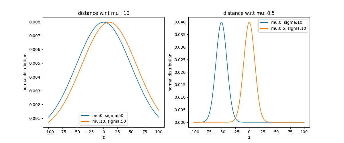
Visually, the first two distributions are similar, while the other two barely overlap. However, the canonical Euclidean distance with respect to $\mu$ suggests the opposite.
The Euclidean gradient is sometimes not well adapted to VI.
The solution : Natural Gradient, a Riemanian gradient
As explained in this paper, the solution is to define a gradient in a Riemannian space using a symmetric version of the KL divergence. This solution is also discussed in the Stochastic VI paper.
This gradient is called the Natural Gradient and is denoted by $\nabla^{\text{natural}}=\mathcal{I}^{-1}(q) \cdot \nabla$.
It is the product of the inverse of the Fischer matrix and the original gradient.
This leads to the definition of the Natural Gradient Ascent VI, which incorporates the normal gradient into its formula.
Here is a summary of the VI methods to obtain the posterior distribution from the ELBO: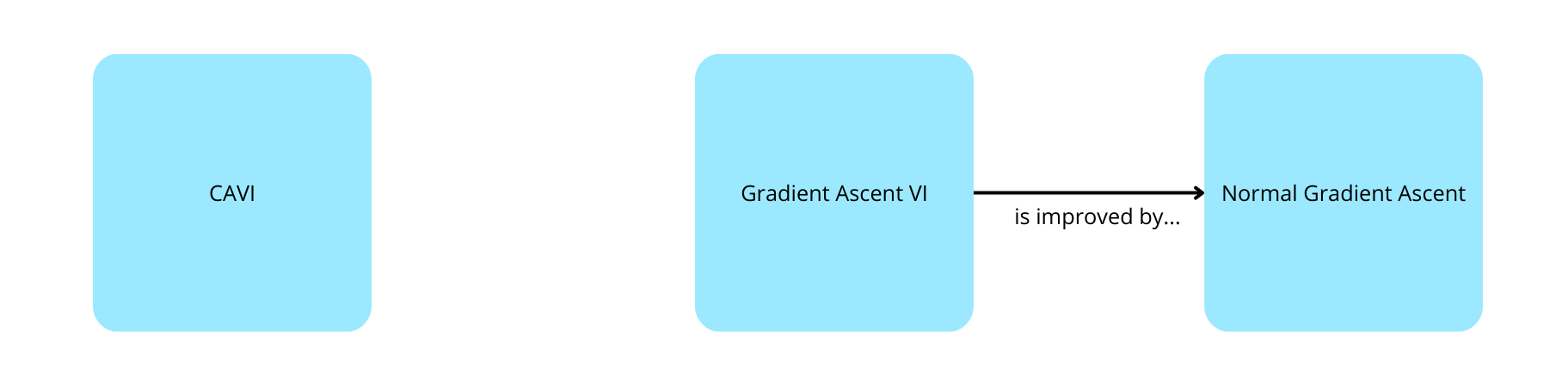
How to compute ELBO gradients ? Is there a trick ?
As in Gradient Ascent VI, the Normal Gradient is easy to compute with an exponential family; however, approximating distributions with complex models complicates the calculations.
The difficulty arises from deriving the integral (since expectation is an integral) for the gradient with respect to $\phi$ :
$$\nabla_\phi \textbf{ELBO} = \nabla_\phi \mathbb{E}_{q_\phi(z|x)}(\log{q_\phi(z|x)}-\log{p_\theta(x|z)}.p_\theta(z))$$To simplify the computation we use the log-derivative trick.
It can be shown that :
$$\nabla_\phi \textbf{ELBO} = \mathbb{E}_{q_\phi(z|x)}[(\log{p_\theta(x|z)}.p_\theta(z)-\log{q_\phi(z|x)}).\nabla_\phi \log{q_\phi(z|x)}]$$With this trick, the gradient is applied only to $\log{q(z)}$.
Then the gradient is computed with the Monte-Carlo method from sample of $q(z)$. This calculation is feasible because at a fixed time, $q(z)$ is known.
In summary, the ELBO’s gradient with respect to $\phi$ takes the following approximation in the general case:
$$\nabla_\phi \textbf{ELBO}(x^k) \approx \frac 1 S \sum_i{(\log{p_\theta(x^k|z_i)}.p_\theta(z_i)-\log{q_\phi(z_i|x^k)}).\nabla_\phi \log{q_\phi(z_i|x^k)}} \\ z_i \sim q $$This formula provides a stochastic approximation of the gradient. We will see that this kind of stochastic approach can be extended to improve VI.
Finally, to compute the ELBO’s gradient with respect to $\theta$, we only have to apply the gradient to the expectation:
$$\nabla_\theta\textbf{ELBO}(x^k)\approx-\sum_i\nabla_\theta [\log p_\theta(x^k,z_i)] $$Stochastic VI and Limitations of classic VI algorithms
The main drawback of classic VI is that each substep and iteration requires processing the entire dataset.
An intuitive improvement is to use mini-batches, which introduces stochastic behavior.
Consequently, we adapt Coordinate Ascent VI (CAVI) and Gradient Ascent VI to their stochastic versions, which apply the same algorithms but use mini-batches instead of the entire dataset.
If you are not familiar with mini-batches methods you can check this link.
This leads to Stochastic Variational Inference (SVI), which is more scalable and better suited to large datasets.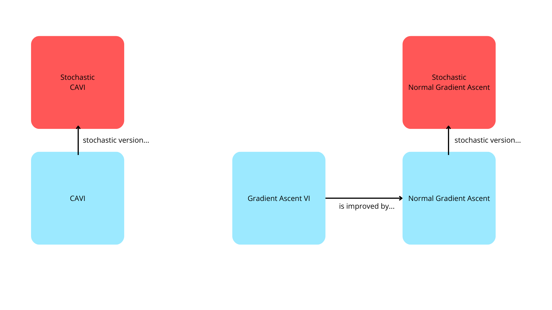
By combining mini-batches with a stochastic approximation of the gradient, we develop a comprehensive method of Stochastic Variational Inference that operates on complex models without requiring the mean-field assumption: Black-Box VI.
You can read the original paper here : BBVI.
The BBVI optimizes the ELBO with the following algorithm :
- Choose a statistical model and a family distribution for $q_\phi(z|x)$. Initialize with random values for $\phi$ and $\theta$.
- Draw samples $\{z_i\}$ from $q_\phi(z|x)$
- Apply the
log-derivative trickandMonte-Carlo methodto estimate the gradient : $$\nabla_\phi \textbf{ELBO}(x^k) \approx \frac 1 S \sum_i{(\log{p_\theta(x^k|z_i)}.p_\theta(z_i)-\log{q_\phi(z_i|x^k)}).\nabla_\phi \log{q_\phi(z_i|x^k)}}\\ \nabla_\theta\textbf{ELBO}(x^k)\approx-\sum_i\nabla_\theta [\log p_\theta(x^k,z_i)]$$ - Construct
mini-batcheswith your dataset and refresh the $\theta$ with : $$\theta^{t} = \theta^{t-1}+\alpha^t.\nabla_\theta\textbf{ELBO} \\ \phi^{t} = \phi^{t-1}+\alpha^t.\nabla_\phi\textbf{ELBO}$$
However, this method’s flexibility often results in high variance.
To address this, the paper suggests solutions such as Rao-Blackwellization and control variates methods. The last one is introduced in this paper.
You can read the BBVI paper to see updated algorithms.
Conclusion about VI
In conclusion, we have seen that Variational Inference provides algorithms to approximate posterior distributions. These algorithms approach this approximation as an optimization problem. The objective function for optimization is the Evidence Lower Bound (ELBO).
However, with large datasets, VI algorithms become computationally demanding.
Additionally, gradient-based algorithms rely on strong assumptions that are not always appropriate.
This led to the development of Stochastic Variational Inference (SVI), where algorithms like BBVI perform well despite high variance.
In the third part of this article, we will explore how this technology has become central to generative AI. The key lies in leveraging an Autoencoder architecture trained with Variational Inference following principles similar to BBVI.
II. Auto-Encoder
Auto-Encoder is a type of neural network architecture that represents a specific case of the Encoder-Decoder framework.
Today, encoder-decoder architectures are at the forefront of major challenges in deep learning. Let’s do a quick recap of these architectures.
From Encoder-Decoder to Auto-Encoder
Encoder-Decoder networks are neural networks suited for sequence-to-sequence tasks. They consist of two main components:
Encoder: processes the input and creates a fixed-size representation (known as anembedding) in a latent space, aiming to capture the essential information.Decoder: uses the embedding as input and generates an output step-by-step from it.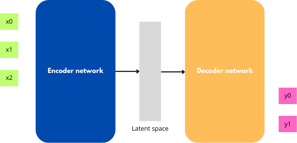
Figure 5 : An encoder-decoder architecture.
For instance, if we have a 28x28 pixel image containing a circle, it can be compressed into a 3D vector representing the center position and radius of the circle. This is the role of the encoder.
Then, using these latent variables, the decoder can infer information such as whether the circle’s area exceeds a certain threshold.
The Auto-Encoder is essentially an encoder-decoder architecture, except its objective is to reconstruct the encoder’s input $x$.
If I give $x$ as input to the model, I want $x$ as the decoder’s output.
In the example of the circle image, the decoder would generate a circle with the appropriate radius and center position.
At first glance, this may seem unhelpful. However, this concept enables tasks such as:
- Image reconstruction
- Image denoising
- Learning compression
For instance, in document compression, the document $d$ is passed through the encoder. This results in a compressed representation of the document in the latent space.
Since the encoder retains only the key information, the document is now compressed.
The decoder can then reconstruct the document using the auto-encoder principle: the encoder input is also the decoder output.
Can data be generated once the latent space is built?
Let’s consider an auto-encoder trained for image reconstruction with a latent space $Z$.
What if we take a random point $z \in Z$ and pass it to the decoder to generate an image?
The produced image will likely be incoherent because the latent space generated by an auto-encoder is unstructured.
This is true even if we choose a $z_0$ point near a $z_1$ point that represents a real, coherent image.
In conclusion, if our goal is data generation, we need to build an organized and continuous latent space.
III. Variational Auto-Encoder (VAE)
Variational Auto-Encoder (VAE) is an enhancement of the traditional auto-encoder achieved through Stochastic Variational Inference.
We train VAEs by constraining the latent space to approximate a fixed distribution using variational inference methods. This results in a more continuous and organized latent space.
We model the VAE and the data as follows: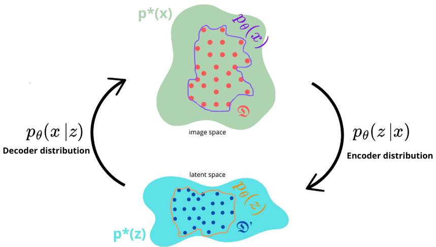
- The input dataset $ \mathcal{D} $ and its corresponding representation in the latent space, $ \mathcal{D'} $
- $ p_\theta(x) $: the modeled distribution of the dataset images in the input space, and $p_\theta(z)$: the modeled distribution of the latent variables in the latent space.
- $p_\theta(z|x)$: the distribution mapping the input space to the latent space, and $p_\theta(x|z)$: the distribution mapping the latent space to the output space.
Using similar notation, we denote the true distributions as $p^*(x)$ and $p^*(z)$.
We aim to approximate $p_\theta(z|x)$ with $q_\theta(z|x)$ using variational inference, seeking to maximize the ELBO.
The VAE paper introduces a method for computing the ELBO gradient with reduced variance, known as the reparametrization trick. As a result, the training algorithm differs slightly from that of BBVI. (see paper).
Reparametrization trick
As with BBVI, the main issue lies in calculating the gradient with respect to ( \phi ). Specifically, we have:
$$ \nabla_\theta\textbf{ELBO}(x^k) \approx -\frac{1}{S} \sum_i \nabla_\theta [\log p_\theta(x^k, z_i)] $$$$ \nabla_\phi\textbf{ELBO}(x^k) = \mathbb{E}_{q_\phi(z|x^k)} \left[\nabla_\phi \left(\log p_\theta(z, x^k) - \log q_\phi(z|x^k) \right)\right] + \int_z \left(\log p_\theta(z, x^k) - \log q_\phi(z|x^k) \right) \nabla_\phi q_\phi(z|x^k) \, dz $$The gradient with respect to ( \phi ) is not expressed as a simple expectation and becomes intractable due to the stochastic nature of ( q_\phi(z|x) ).
To address this, we introduce a differentiable transformation that separates the stochastic component from the gradient:
$$ z = T(\epsilon, \phi)\\ \epsilon \sim \mathcal{p}(\epsilon) $$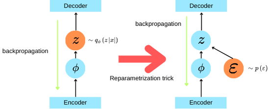
Monte Carlo estimator to approximate the ELBO’s gradient:
Training VAE in practice
Now we know how to compute the gradient of the ELBO using the reparametrization trick.
The idea of a VAE is to construct the latent space by considering the encoder and decoder functions as probability distributions.
It is then possible to construct the latent space with variational inference.
The network’s loss function is the ELBO rewritten in its appropriate machine learning form:
$$\textbf{ELBO} = \mathbb{E_{q_\phi(z|x)}}(\log{p_\theta(x|z)})-\textbf{KL}(q_\phi(z|x)||p_\theta(z))$$We have to set 3 distributions: $p_\theta(z)$, the distribution of the latent space; $p_\theta(x|z)$, the likelihood (or here the decoder distribution); and $q_\phi(x|z)$, the approximate posterior (or here the encoder distribution).
Choice of $p_\theta(z)$ for the training:
Once $p_\theta(z)$ is set, the latent data will be distributed according to this distribution.
We want a continuous space, so the natural choice is to set $p_\theta(z) \sim \mathcal N(0,1)$.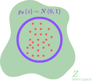
Choice of $q_\phi(z|x)$ for the training:
Since $p_\theta(z)$ is Gaussian, we will have an analytical solution for the $\textbf{KL}(q_\phi(z|x)||p_\theta(z))$ term if we choose $q_\phi(z|x) \sim \mathcal{N(z|\mu(x),\sigma^2(x))}$.
As a consequence, we have with calculus: $\textbf{KL}(q_\phi(z|x)||p_\theta(z)) = -\frac 1 2(\log\sigma^2-\mu^2-\sigma^2+1)$.
Choice of $p_\theta(x|z)$ for the training:
This distribution will determine the output distribution.
This choice depends on the type of images we are working with. For example, if our dataset is MNIST, we will choose a Bernoulli distribution. However, if our dataset is the Iris dataset, we will choose a continuous natural distribution, like a Gaussian.
For this article, we will choose a Gaussian: $p_\theta(x|z) \sim \mathcal N(y_\mu, y_\sigma^2)$.
To reduce the variance in the output, we set $y_\sigma=1$.
Thus, the expectation term in the ELBO loss function becomes: $\mathbb{E_{q_\phi(z|x)}}(\log{p_\theta(x|z)})=-\log\sqrt(2\pi)-(x-y_\mu)^2$.
Up to an additive constant, $\mathbb{E_{q_\phi(z|x)}}(\log{p_\theta(x|z)})=(x-y_\mu)^2$.
Amortized Variational Inference
Rather than considering the distribution $q_\phi$ as the output of the encoder, we consider parameters like $\mu$ and $\sigma$ as the output of the encoder.
The encoder becomes a function $f$ that maps data $x$ to $(\mu, \sigma)$.
The advantage is that we don’t need to recompute the map $x \rightarrow (\mu, \sigma)$ when we add new samples to the batch.
This method is called amortized variational inference.
Thus, the expectation term in the ELBO loss function becomes deterministic and corresponds to the MSE loss between the original data and the expectation of $p_\theta(x|z)$.
As a consequence, a VAE is an encoder-decoder model where the encoder learns $\mu$ and $\sigma$.
These parameters are learned through a dataset $\mathcal D$ and the ELBO loss function:
The gradient is computed with the reparametrization trick and then is updated with an optimizer on parameters of distributions.
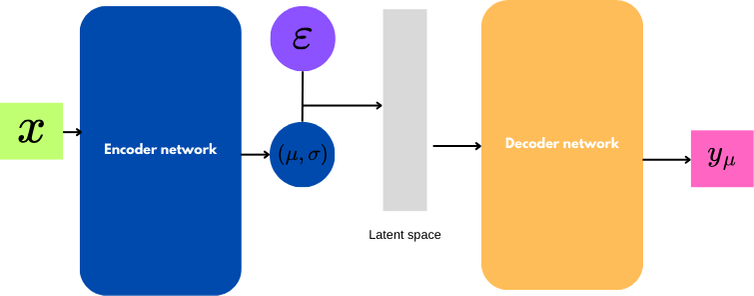
A typical forward pass involves feeding the encoder an image $x$, after which the encoder produces $\mu$ and $\sigma$.
Then we sample $\epsilon$, and we have a $z$ sampled.
We feed this $z$ into the decoder, and the decoder produces an output $y$.
This training produces a latent space that is continuous and organized compared to classic auto-encoders.
If we want to generate an image $x'$ that resembles an original image $x$, I just need to get $\mu(x), \sigma(x)$ and then sample $\epsilon$. Then we get $z'=\mu+\epsilon.\sigma$. If we just want to generate a random image, we sample $z$ from $p(z)$, which is a unit gaussian.
This latent variable could be used in the decoder to produce a new image.
Limits of VAE
With the theory above, it seems that VAEs are perfect for generating images. They have a continuous and well-organized latent space, so why do they face challenges in practice?
Here is a sample of faces generated by VAEs:
All the images are blurry. Why?
One explanation is that the ELBO loss function is unbalanced between KL divergence, which tries to fit the latent space to a normal distribution, and the reconstruction loss like MSE.
Due to the stochasticity of the latent space during training, one sample could produce a distribution of slightly different $z$ values. Because of this difference, the reconstruction loss tries to average the variations, which is a mathematical model for blurriness.
Thus, the model underfits sharper details.
Moreover, the latent space produced is not flexible enough to generate precise outputs.
Since the first VAE paper, many proposals for improving generation quality have been suggested.
$\beta$-VAE
An improvement of VAEs is to set a $\beta$ hyperparameter in the loss function to balance the reconstruction loss and KL divergence. This idea is proposed by Higgins et al. (2017). They propose a new form of the ELBO loss function:
$$\mathcal{L} = \mathcal{L}_\text{reconstruction} - \beta \cdot \textbf{KL}(q_\phi(z|x)|| p_\theta(z))$$The reconstruction loss could be an L2 loss.
If we choose $\beta > 1$, the distribution $q_\phi(z|x)$ is encouraged to match the prior $p_\theta(z)$, which is a unit Gaussian. Thus, the reconstruction loss has only a slight impact on the result, which helps avoid blurry images during generation. The main drawback is that it reduces the mutual information between a point $z$ and a point $x$.
Moreover, $\beta$-VAE promotes the disentanglement of the latent space.
What is a disentangled latent space? The idea of a latent space is to produce a space with a smaller dimension than the data space. A latent space offers the possibility to encode data with a few parameters.
For instance, an image of a circle could be encoded with 3 dimensions: the position of the center and the radius. Here, the latent space has two dimensions for the position and one for the radius. Now if we want to generate a circle, we could choose a center position and a radius.
This is a disentangled latent space: each dimension represents a specific feature, and each feature is independent.
However, standard VAEs do not produce disentangled latent spaces.
The paper Understanding disentangling in $\beta$-VAE explains why a $\beta > 1$ helps the disentanglement of the latent space.
This paper proposes an analogy between VAEs and a noisy communication channel in information theory.
The original image $x$ is the input, and the latent variable $z$ is the output.
Thus, we want to estimate the channel capacity of a VAE:
The paper states that high capacity produces less regularization during training. Then, latent representations become more complex and do not produce independent latent channels. However, with a smaller capacity, we enforce higher regularization, which then produces independent latent channels.
To balance the benefits of disentanglement with good reconstruction quality, Higgins et al. introduced a new training method for $\beta$-VAE. Since it is possible to control the capacity with the KL divergence, we apply high regularization in the first iterations, encouraging disentanglement in the early stages of training. Then we increase the capacity to capture details through the reconstruction loss.
This leads to a new version of the loss function:
$$\mathcal{L} = \mathcal{L}_\text{reconstruction} - \gamma [\textbf{KL}(q_\phi(z|x)|| p_\theta(z)) - C]$$The $\gamma$ is the new hyperparameter (previously called $\beta$) and $C$ is the channel capacity, which increases gradually.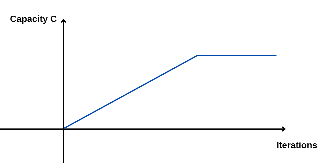
Is there a quantitative link between low capacity and disentanglement?
Chen et al. (2018) propose, in Isolating sources of disentanglement in VAEs, a decomposition of the KL divergence term as follows:
$$ \mathbb{E}[\textbf{KL}(q_\phi(z|x), p_\theta(z))] = \textbf{KL}[q_\phi(z,n)||q_\phi(z) \cdot p_\theta(n)] + \textbf{KL}[q_\phi(z)||\Pi_j q_\phi(z_j)] + \sum_j \textbf{KL}[q_\phi(z_j)||p_\theta(z_j)] \\ \mathbb{E}[\textbf{KL}(q_\phi(z|x), p_\theta(z))] = \text{image-latent mutual information} + \text{total correlation} + \text{KL dimension-wise}$$This decomposition highlights that disentanglement is only a part of the KL divergence. This property is measured by the total correlation term.
To target disentanglement, the authors propose the \beta-TCVAE (Total Correlation VAE), which sets hyperparameters in the loss function:
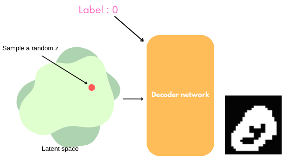
Conditional VAE
Conditional VAE (CVAE) proposes introducing multi-modality to generate more precise elements.
With a classic VAE, we sample a random $z$ and generate an image using the decoder.
But what if we want to generate a specific image?
For instance, with the MNIST dataset, how do we proceed to generate a 6 or a 3?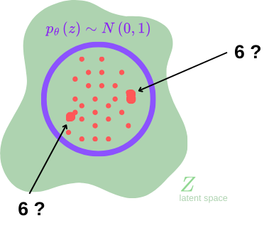
The contribution of the CVAE lies in the addition of a label $c$ during the training and generation steps.
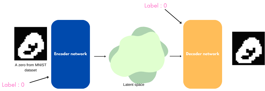
Thus, the generation step follows this principle:
VQ-VAE
VAEs generate a continuous normal distribution for data $x$ with the encoder. Then we sample a $z$ over this distribution and pass it through the decoder.
However, the standard VAE framework ignores the potential sequential structures in the data. Moreover, for certain modalities like language, continuous posterior and prior distributions are not suitable.
Here is the starting point of van den Oord et al. in the VQ-VAE paper.
Their research focuses on the development of a VAE with a discrete latent space and an auto-regressive prior.
This is the architecture proposed: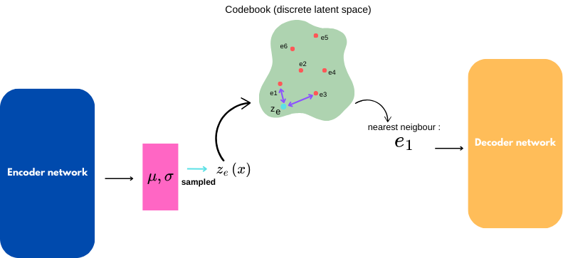
They choose a cardinality $K$ for the discrete latent space and a dimension $D$ for the embeddings.
The encoder works as in classic VAEs. The sampled $z_e$ is passed through the codebook, and a nearest-neighbor algorithm is applied.
However, it is impossible to backpropagate a gradient through the codebook. The VQ-VAE paper chooses to skip this non-linearity and sends the gradient from the decoder’s input to $z_e$.
To train the codebook, a regularization term with a skip-gradient function is added. During backpropagation, this term is set to zero.
The new loss function is:
$$\mathcal{L}_{\text{vq-vae}} = \mathcal{L}_{\text{reconstruction}}+||\text{sg}[z_e]-e||^2_2+\beta||z_e-\text{sg}[e]||^2_2$$The regularization term $||\text{sg}[z_e]-e||^2_2+\beta||z_e-\text{sg}[e]||^2_2$ updates the discrete embeddings and attracts $z_e$ to the discrete embeddings to stabilize training.
Once training is complete, they use an external auto-regressive model to fit a prior distribution $p$ over the latent space.
Thus, the prior is not a simple Gaussian.
Hierarchical VAE
So far, we have presented VAEs with only a single network.
It is natural in deep learning to try a deep VAE. The goal could be to construct a latent space with increasing precision. This approach could help avoid blurriness in generation.
Nevertheless, is it possible to build multi-level VAEs to achieve better results?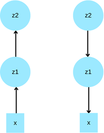
Sonderby et al. demonstrate that Batch Normalization and Warm-up (a technique which increases the importance of KL over epochs) improve the performance of naive hierarchical VAEs.
To stabilize Hierarchical VAEs, Ladder VAE proposes coupling posterior and generative distributions. NVAE proposes using residual blocks and skip connections.
Ladder VAE: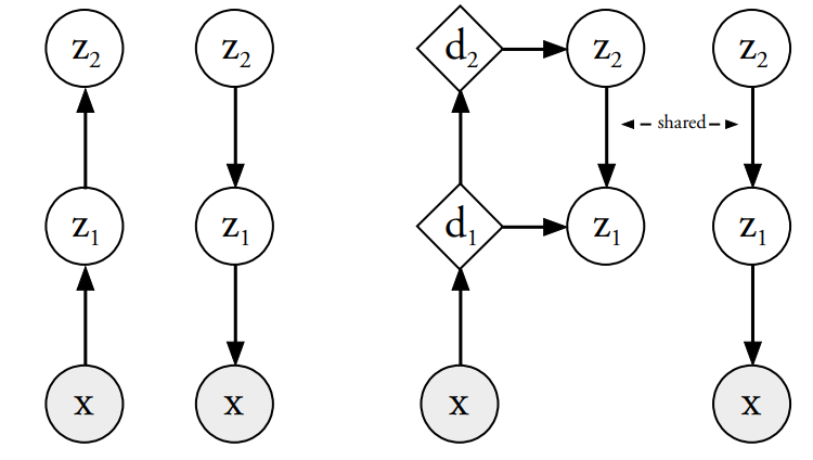
Sonderby et al. (2016) propose using the parameters of $p_\theta(x|z)$ at a layer $i$ to reparameterize the distribution $q_\phi(z|x)$ at layer $i$.
$$\begin{align*} q_\phi(\mathbf{z}|\mathbf{x}) &= q_\phi(z_L|\mathbf{x}) \prod_{i=1}^{L-1} q_\phi(z_i | z_{i+1}) \\[10pt] \sigma_{q,i} &= \frac{1}{\hat{\sigma}_{q,i}^{-2} + \sigma_{p,i}^{-2}} \\[10pt] \mu_{q,i} &= \frac{\hat{\mu}_{q,i} \hat{\sigma}_{q,i}^{-2} + \mu_{p,i} \sigma_{p,i}^{-2}}{\hat{\sigma}_{q,i}^{-2} + \sigma_{p,i}^{-2}} \\[10pt] q_\phi(z_i | \cdot) &= \mathcal{N}(z_i | \mu_{q,i}, \sigma_{q,i}^2) \end{align*}$$As such, LVAE helps the encoder and decoder communicate together. The paper draws an analogy to a human analyzing an image. Natural perception involves back-and-forth processing between the real signal and brain signal.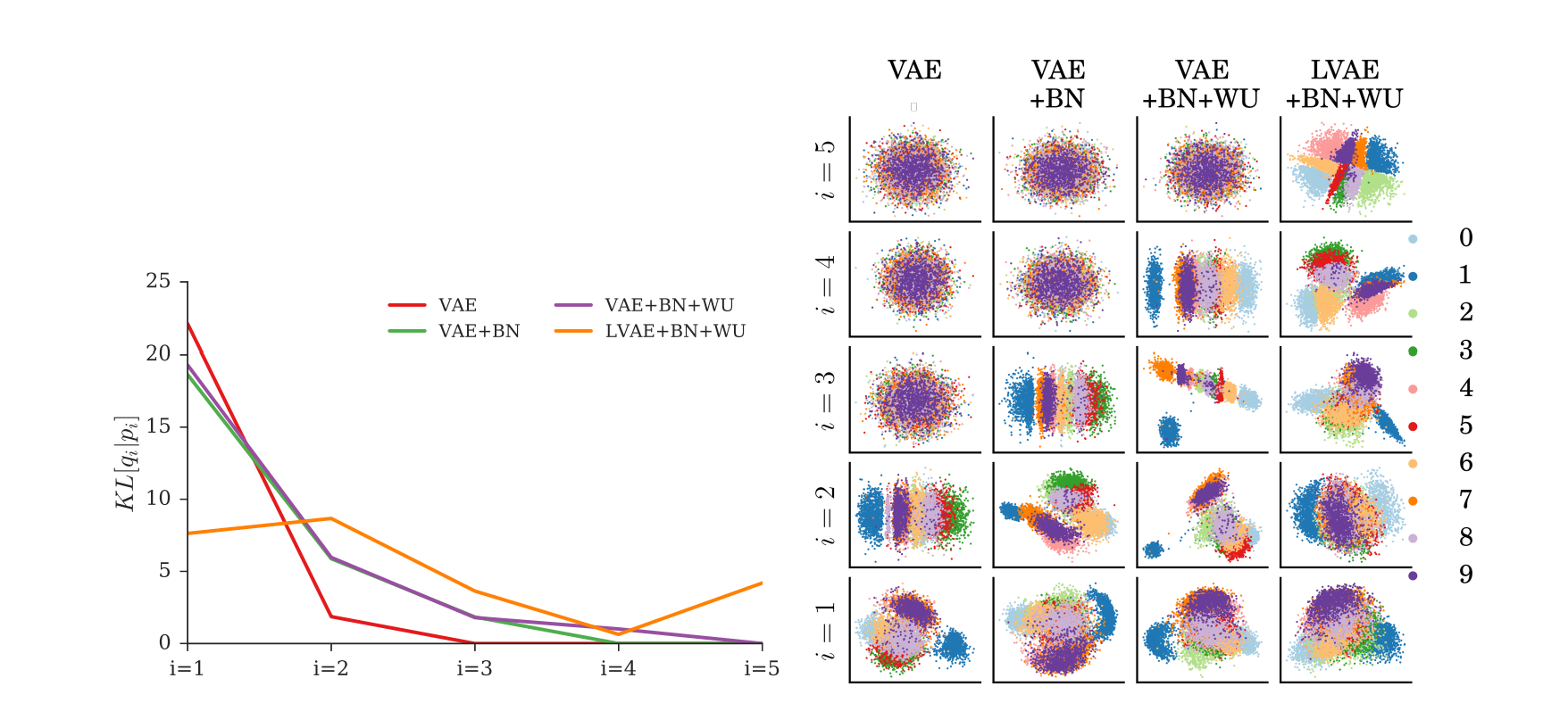
Finally, LVAE focuses training on each layer and produces a well-organized latent space.
However, the datasets used in experiments with Ladder VAE are simple image datasets, like MNIST and OMNIGLOT, which contain symbols.
Models like Nouveau VAE are tested on more complex tasks, such as image generation.
Nouveau VAE: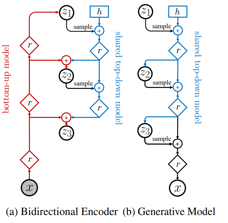
NVAE (Vahdat et al.) proposes constructing a latent space with multi-level precision using residual cells.
The residual cells in the encoder upcast the dimension of images to capture more detailed information with a 1x1 convolutional layer.
To stabilize training, batch normalization and two additional techniques are used:
Reparameterization of $q$ at a level $l$ using information from the prior distribution. Let $p(z_l^i|z_{\lt l})$ be the prior of the $i$-th variable at layer $l$.
We have $p(z_l^i|z_{\lt l}) \sim \mathcal{N}(\mu_i(z_{\lt l}), \sigma_i(z_{\lt l}))$. We denote $\Delta\mu_i$ and $\Delta\sigma_i$ as the relative parameters, which measure the difference between prior and posterior parameters.
Now we have the posterior distribution:
$$q\left( z_l^i \middle| z_{\lt l}, \mathbf{x} \right) = \mathcal{N} \left( \mu_i(z_{\lt l}) + \Delta \mu_i(z_{\lt l}, \mathbf{x}), \, \sigma_i(z_{\lt l}) \cdot \Delta \sigma_i(z_{\lt l}, \mathbf{x}) \right)$$Spectral regularization: A regularization term is added to the loss function:
$$\mathcal{L}_\text{SR} = \lambda \Sigma_i s^{(i)}$$Where $s^{(i)}$ is the largest singular value of the $i$-th layer, and $\lambda$ is a hyperparameter.
The final loss is:
$$\mathcal{L}_{\text{VAE}}(x) = \mathbb{E}_{q(z|x)} \left[ \log p(x|z) \right] - \text{KL}\left(q(z_1|x) || p(z_1)\right) - \sum_{l=2}^{L} \mathbb{E}_{q(z_{\lt l}|\mathbf{x})} \left[\text{KL}\left(q(z_l|\mathbf{x}, z_{\lt l}) \parallel p(z_l|z_{\lt l})\right)\right] + \mathcal{L}_\text{SR}$$Conclusion
We have seen that Variational Inference methods help us approximate distributions by minimizing the Evidence Lower Bound using the Kullback-Leibler divergence and algorithms like CAVI or BBVI. VI introduces tricks to compute gradients efficiently, such as the log-derivative trick or reparameterization trick.
In generative deep learning, VI allows us to construct stochastic latent spaces, which are more continuous than deterministic latent spaces.
This leads to models such as Variational Auto-Encoders. These kinds of models have limited generation capacity compared to auto-regressive models or GANs.
However, modifications to the architectures and loss functions help VAE-like models become competitive, state-of-the-art models in data generation.
Moreover, VAE-like models produce a latent space, not just a black-box generator. These models are suitable for encoding tasks.
This article is the first stage of a project in my final year of engineering studies. I will study the training of NVAE and then use it to improve cardiac shape segmentation.
Bibliography
[1] : David M. Blei, Alp Kucukelbir, Jon D. McAuliffe (2018), Variational Inference : a review for statisticians
[2] : Kaiwen Wu, Jacob R. Gardner (2024), Understanding Stochastic Natural Gradient Variational Inference
[3] : Matt Hoffman, David M. Blei, Chong Wang, John Paisley (2013), Stochastic Variational Inference
[4] : Sushant Patrickar, Medium article 2019, Batch, Mini Batch & Stochastic Gradient Descent
[5] : David Wingate, Theo Weber (2013), Automated Variational Inference in Probabilistic Programming
[6] : Diederik P. Kingma, Tim Salimans, Max Welling (2015), Variational Dropout and the Local Reparameterization Trick
[7] : Irina Higgins, Loic Matthey, Arka Pal, Christopher Burgess, Xavier Glorot, Matthew Botvinick, Shakir Mohamed, Alexander Lerchner (2017), beta-VAE: Learning Basic Visual Concepts with a Constrained Variational Framework
[8] : Christopher P. Burgess, Irina Higgins, Arka Pal, Loic Matthey, Nick Watters, Guillaume Desjardins, Alexander Lerchner (2018), Understanding disentangling in β-VAE
[10] : Aaron van den Oord, Oriol Vinyals, Koray Kavukcuoglu (2018), Neural Discrete Representation Learning
[11] : Arash Vahdat, Jan Kautz (2021), NVAE: A Deep Hierarchical Variational Autoencoder
Alexandre MYARA - Oct 2024